Real-time collision detection for Panda with OpenCL

In this blog post I will present a collision detection algorithm specifically tailored for use with Panda. The algorithm was developed as part of my ongoing PhD thesis and later improved by my student Johannes Schwaiger as part of his bachelor’s thesis. The collision detection algorithm is able to analyze point clouds from depth cameras such as Intel Realsense in real-time while a trajectory is executed with the robotic arm. Potential collisions that were not planned to be in the configuration space of the arm and that therefore lie on the current trajectory will be detected and the robotic arm will be stopped immediately by our implementation.

The real-time requirement of this algorithm can only be met with an implementation that offloads computation to a GPU device. We chose to use OpenCL for this purpose. The GPU that we used for testing our algorithm was the AMD Radeon VII with ROCm v5.3 drivers on Ubuntu 20.04. Our implementation is based on OpenCL 2.0 which is to our knowledge currently only supported by AMD on consumer and workstation grade graphics cards. OpenCL Version 2.0 allows writing on 3D image structures directly from within the device code which is one of the key steps in our algorithm.

System Components

The algorithm consists of various components that fullfill different tasks:

• CollisionDetector: Host / CPU code written in C++ as a ROS node. This node coordinates the communication with the rest of the components. It is also responsible for managing the device / GPU interaction and resources.
• MeshReader: ROS node written in C++. This node is responsible for converting the mesh surface data of the robotic arm’s link into 3D volumes.
• SphereVisualizer: ROS node written in C++. This node is solely responsible for visualizing a set of points in the robot’s surroundings in RViz.
• detection.cl: Device / GPU code for determining which points in the point cloud are a potential collision.
• verification.cl: Device / GPU code for deciding if a point in the point cloud that was marked as collision is a collision or just noise resulting form poor measurement accuracy of the depth camera.

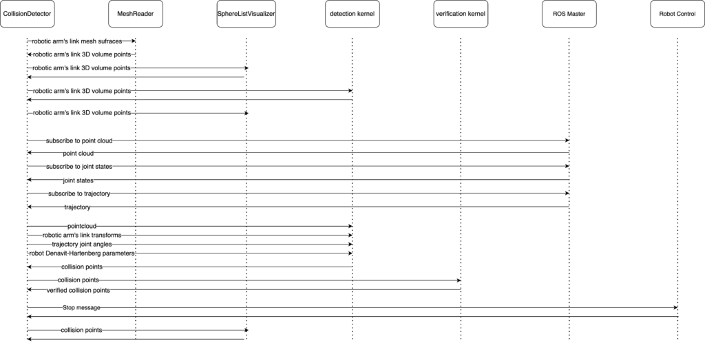
Below you can find a sequence diagram that shows how the components interact with each other.

Robot simulation and environment

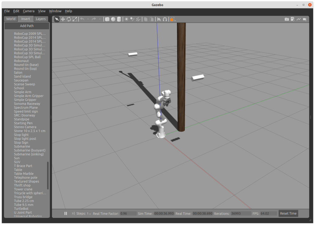
We are simulating the robotic arm in Gazebo next to a potential collision object (a telephone pole). Two depth cameras capture the movements of the robotic arm and send point clouds to our implementation via ROS Master.

Implementation

In the following we will discuss the collision detection procedure in detail.

The procedure starts with the init() method in the CollisionDetector ROS node. It consists of the following steps:

• A set of configuration parameters are read form the ROS master
• The private node parameters that were passed to the node at its launch are read into variables
• The robotic arm’s mesh surface files are converted into volume files. These volume points are filtered / reduced to the most essential points in order to reduce the runtime of the algorithm.
• The kinematics model of the robotic arm is read from the ROS master
• The Denavit-Hartenberg parameters of Panda are set as compile time parameters to the detection OpenCL kernel
• The most essential coordinate transforms are retrieved
• Static data is sent to the GPU device by allocating a buffer for each of the variables. A special case here is the 3D OpenCL image that discretizes the surroundings of the robotic arm into a 3D volume.
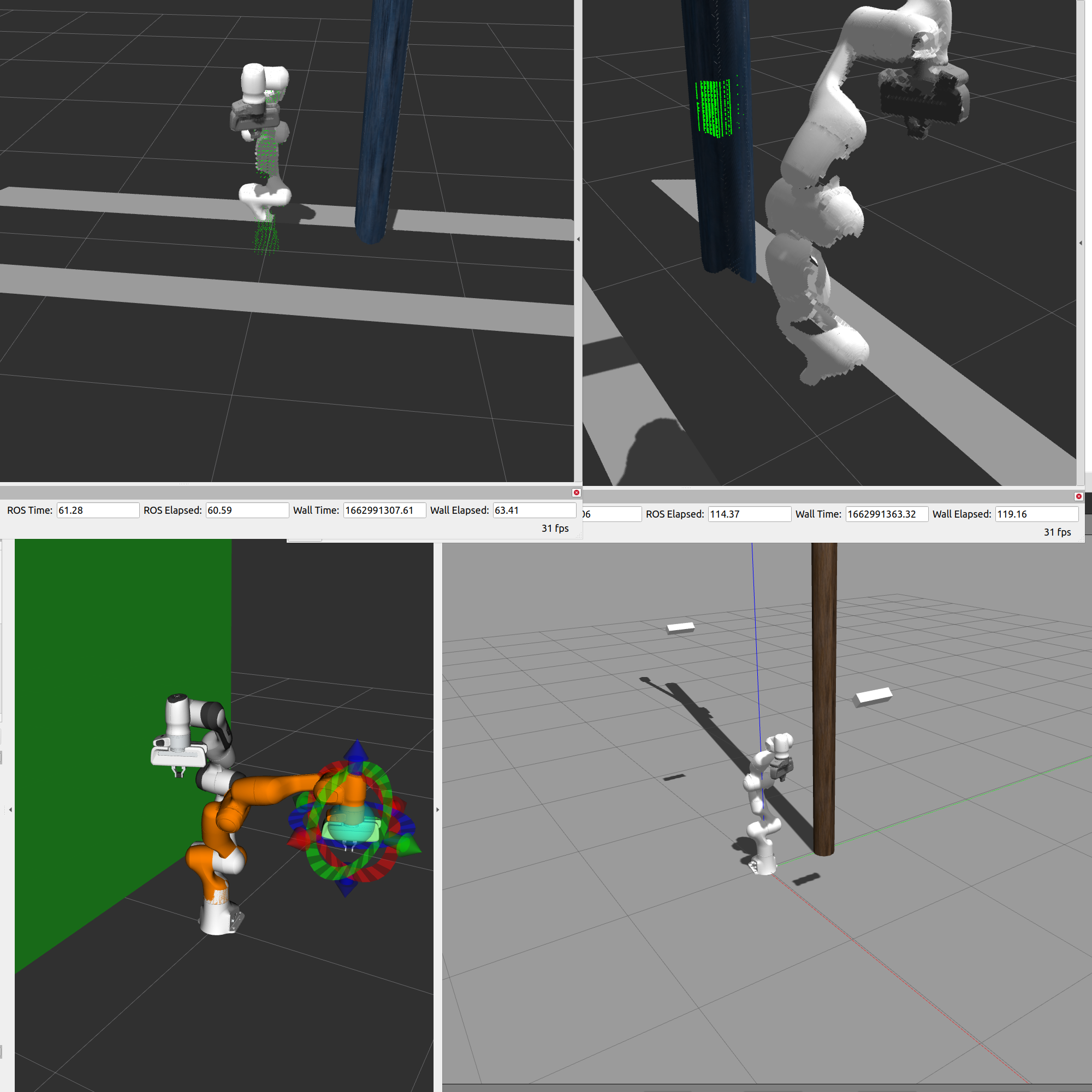
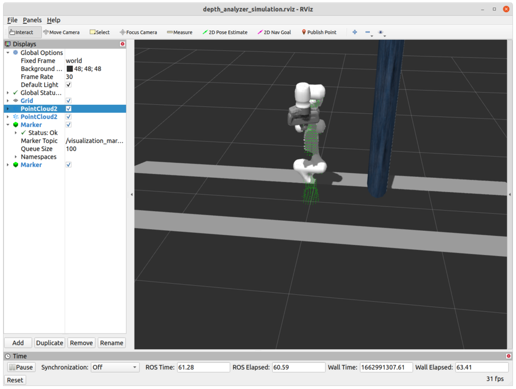
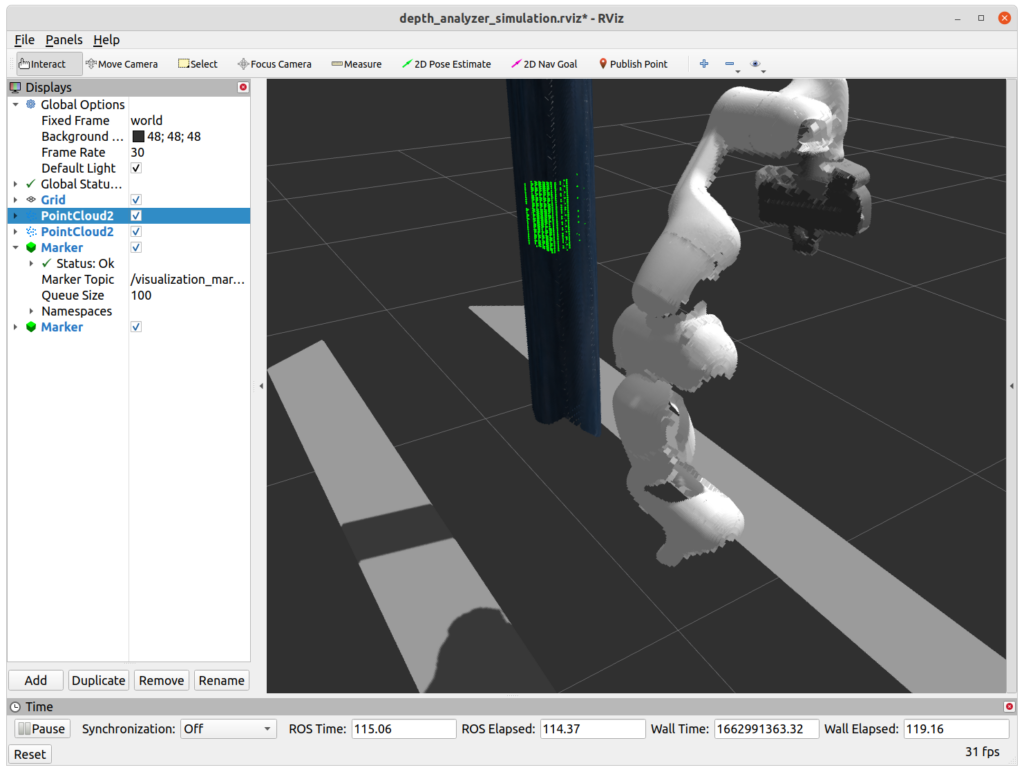
• The robotic arm’s link volume points are sent to SphereListVisualizer for visualization in RViz. This is helpful because in the visualization the mesh surfaces can be checked for proper conversion and placement into the right coordinate frame. Otherwise, the visualization will not show the green markers in the correct shape or at the correct position.

The joint states callback

The joint states callback captures the current state of the robotic arm. In our implementation it serves the purpose of sending the state of the arm to the GPU whenever an update is received. In the simulation the joint state topic publishes at a rate of 30 Hz, which means that the GPU receives an update 30 times per second. The update written asynchronously with to a device buffer.

There is a catch though: we should only use a state of the arm that was captured before the point cloud was captured. If we use a state of the arm that was captured after the point cloud measurement was received than the filter will try to remove the robotic arm from the point cloud at a position that will be captured in the future, meaning in the next frame of the depth camera.

This means that we should store a series of joint states and in advance and use the state that was received just before the point cloud was captured. For this reason we are using an std::deque and an std::map for storing a set of joint states in the right order. The deque data structure provides efficient push and pop operations with the First-In-First-Out (FIFO) principle. We can store and delete joint states in the right order with this data structure: The state of the arm that first entered the deque will also be the first state that leaves the deque when a certain capacity is reached.

The robotic arm’s current state is sent to the GPU as actual transforms in form of 4×4 matrices (rotation + translation) for each link.

The trajectory callback

The trajectory consists of multiple waypoints, where each waypoint consists of 7 angles: one angle for each rotational joint of the robotic arm. We could calculate each link’s transform matrix at each waypoint as we did above with the joint states. This would consume a considerable amount of bandwidth on the GPU though when accessing the device buffer in the kernel code. In fact, we will see later that we have to reduce the amount of data stored in the local memory of the execution units as much as possible. For this reason we employ the Denavit-Hartenberg parameters for the parametrization of the robot states on the trajectory waypoints.

The Denavit-Hartenberg parameters for each link are set as compile-time parameters for the OpenCL kernel except for the parameter theta which describes the angles of the rotational joints at the waypoints is written to the device buffer when the trajectory is received in the respective callback method.

The point cloud callback

The point cloud callback is executed every time a point cloud frame is captured and published by the depth camera in the simulation. The callback checks if a trajectory was received beforehand, because otherwise the robot will stand still and processing the point cloud is not necessary. If a trajectory was received and written to the GPU though, the received point cloud is written to the GPU buffer followed by a series of data transfer calls. The aforementioned selection of the correct state of the robotic arm is also handled in this callback. After pushing all of the necessary arguments to the GPU, the computation on the device is started by launching a thread (also called work-item) for each point in the point cloud.

The first kernel running on the GPU is the detection.cl kernel. This kernel decides which points in the point cloud are a potential collision. In order do that in a reliable manner, the surroundings of the robot are discretized in as a 3D volume. This means that every measurement in meters in the vicinity of the robotic arm is mapped to a voxel in a volume with predefined dimensions (in our case 512 x 512 x 512). When a point in the point cloud is reported as potential collision for the trajectory that is currently executed, we determine its coordinates in the aforementioned discretized volume. This coordinate of the volume is then marked as a potential collision candidate and will be further checked in a later step.

This kind of discretization has the advantage that no magic threshold for the number of potential collision points has to be selected after which we can definitely state that a collision would take place. There might be noisy measurements in the point cloud after all. This threshold would be set in order to distinguish between sensor noise and a definitive collision point.

The second kernel is invoked after receiving the results from the first one. It applies simple neighbourhood checking on the discretized volume and returns a definitive statement on whether there is a collision on the trajectory. The number of collision points is printed to the console.

In case of a collision a stop message is sent to the robot control node in order to interrupt the trajectory execution. The collision points are converted from the discretized volume coordinates to the their original coordinate frame with a meter representation. These coordinates are sent to the SphereVisualizer node where they are published to RViz as 3D markers. The user can see the location of the collision points in RViz.

The detection kernel

The detection kernel has two tasks: Filtering the robotic arm from the given point cloud and checking the remaining points in the point cloud for a collision with the trajectory that is currently being executed.

Robot self-filter

In order to filter the robotic arm from the given point cloud we check the distance of a point from the point cloud to each of the volume points of the robotic arm. The volume points were transferred to the GPU in the point cloud callback. If the distance of the point falls below a given threshold (10 cm) for all of the link volume points, we exit the kernel without further computation. The volume points are placed at the right positions by using the link transforms that were transferred to the GPU whenever a new update update the robotic arm’s joints were received from the simulation.

Collision detection

If the point does not lie within the robotic arm’s estimated position, we check if the it lies on the trajectory that the robotic arm is currently executing. This is done with the following steps:

1. Loop over all trajectory waypoints
2. For every point in the robotic arm’s volume determine it’s position in the current and the next waypoint of the trajectory
3. Check the distance of the given point from the point cloud to the volume point’s location on the current waypoint
4. Check the distance of the given point from the point cloud to the volume point’s location on the next waypoint
5. Check the distance of the given point from the point cloud to a line that connects the volume point’s location on the current and next waypoint
6. If one of these three distances is below a predefined threshold (3 cm) we assume a collision

The third collision check (5.) constructs a cylinder from the volume point’s current and next location on the trajectory. This check ensures that the point from the point cloud does not lie within this cylinder. We try to estimate the motion of this part of the robotic arm in a given timeframe as a linear motion from one point to the other.

If a collision is detected, the coordinates of the given point from the point cloud are converted to its index in a predefined discretized volume. This volume encompasses the robotic arm’s reachable area. The discretized volume is maintained as an OpenCL 3D image on the device, hence we set the value at the index that we calculated earlier to 1 in order to indicate that this part of the volume contains a collision.

The verification kernel

The verification kernel makes sure that the reported collisions in the discretized volume are not just noisy measurements but actual collisions. If and only if all neighbours of a given collision voxel are also collision voxels it confirms that there is a collision. The result is written to a flat array with the discretized volume’s size.

Results

We simulated the robotic arm together with two depth cameras in the Gazebo simulation environment and for the collision checks we placed a telephone pole next to the arm.

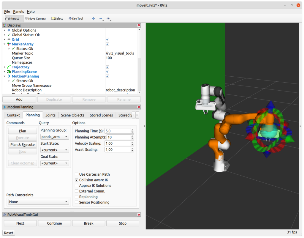
For the collision check we planned a trajectory to a goal that is very close to the potential collision object (the telephone pole) with MoveIt! on the RViz user interface.

Performance evaluation

The collision nodes can be started with the visualize flag in order to get more debugging information on the console and in RViz. When this feature is enabled the collision detection runs slower as more data is transmitted between the CPU and the GPU for visualization purposes. Each frame of the point cloud is processed in 150 milliseconds on average.

When the visualization is disabled we have an average processing time of 35 millisecons per camera frame. These numbers were measured on a workstation with a compatible AMD Radeon VII GPU running two independent collision detection processes simultaneously, one per depth camera.

The custom ROS package as well as the modified franka_ros repository that is needed for the simulation are available in my GitHub profile.